
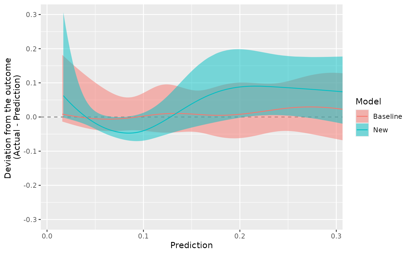
ggcalibrate_BA plots the deviation of the actual event rate from the stats::predicted events (Actual - Prediction) against the prediction, similar to a Bland-Altman plot.
Arguments
- x1
Either a logistic regression fitted using glm (base package) or lrm (rms package) or calculated probabilities (eg through a logistic regression model) of the baseline model. Must be between 0 & 1
- x2
Either a logistic regression fitted using glm (base package) or lrm (rms package) or calculated probabilities (eg through a logistic regression model) of the new (alternative) model. Must be between 0 & 1
- y
Binary of outcome of interest. Must be 0 or 1 (if fitted models are provided this is extracted from the fit which for an rms fit must have x = TRUE, y = TRUE).
- n_knots
The curves are made by fitting a restricted cubic spline (rms package). The default 5-knots is usually enough.
- ci_level
Confidence interval of the curve (default = 0.95).
- alpha_level
Transparency (alpha) of the shaded confidence interval (default = 0.25).
Details
Perfect calibration is the horizontal line at zero. A curve above the line means the model under-predicts the outcome, and a curve below it means the model over-predicts. The curves and confidence intervals are the same as in [ggcalibrate()], with the prediction subtracted. To focus on the region of interest (eg around a decision threshold), add `coord_cartesian(xlim = ...)` to the plot.
Examples
# Quick example with subset of data
data(data_risk)
data_subset <- data_risk[1:100, ] # Use first 100 rows for speed
complete_cases <- complete.cases(data_subset)
data_clean <- data_subset[complete_cases, ]
y <- data_clean$outcome
x1 <- data_clean$baseline
x2 <- data_clean$new
output <- ggcalibrate_BA(x1, x2, y, n_knots = 3, ci_level = 0.95, alpha_level = 0.25)
# \donttest{
# Full dataset example
data(data_risk)
complete_cases <- complete.cases(data_risk)
data_clean <- data_risk[complete_cases, ]
y <- data_clean$outcome
x1 <- data_clean$baseline
x2 <- data_clean$new
output <- ggcalibrate_BA(x1, x2, y, n_knots = 5, ci_level = 0.95, alpha_level = 0.5)
# Zoom in on predictions below 30%
output + ggplot2::coord_cartesian(xlim = c(0, 0.3), ylim = c(-0.3, 0.3))
#> Coordinate system already present.
#> ℹ Adding new coordinate system, which will replace the existing one.
 # }